Over Christmas, I’ve spent a fair bit of time playing board games with my family. However, being me, I can never just play a game without also exploring the maths behind it, much to my family’s general annoyance.
In this post, I’ll be looking at a simple game that we played and how we can use Markov chains to analyse it. Finally, we’ll discover just how much of an advantage the youngest player, who starts first, has.
The Game
My sister is learning to drive at the moment, and as a bit of a joke one of her presents was a board game called “Road Safety Game” (really catchy name indeed). To our amusement, the game was nothing more than Snakes and Ladders with the riveting new rule that “when you land on a snake or a ladder, you have to read out some road safety message”.
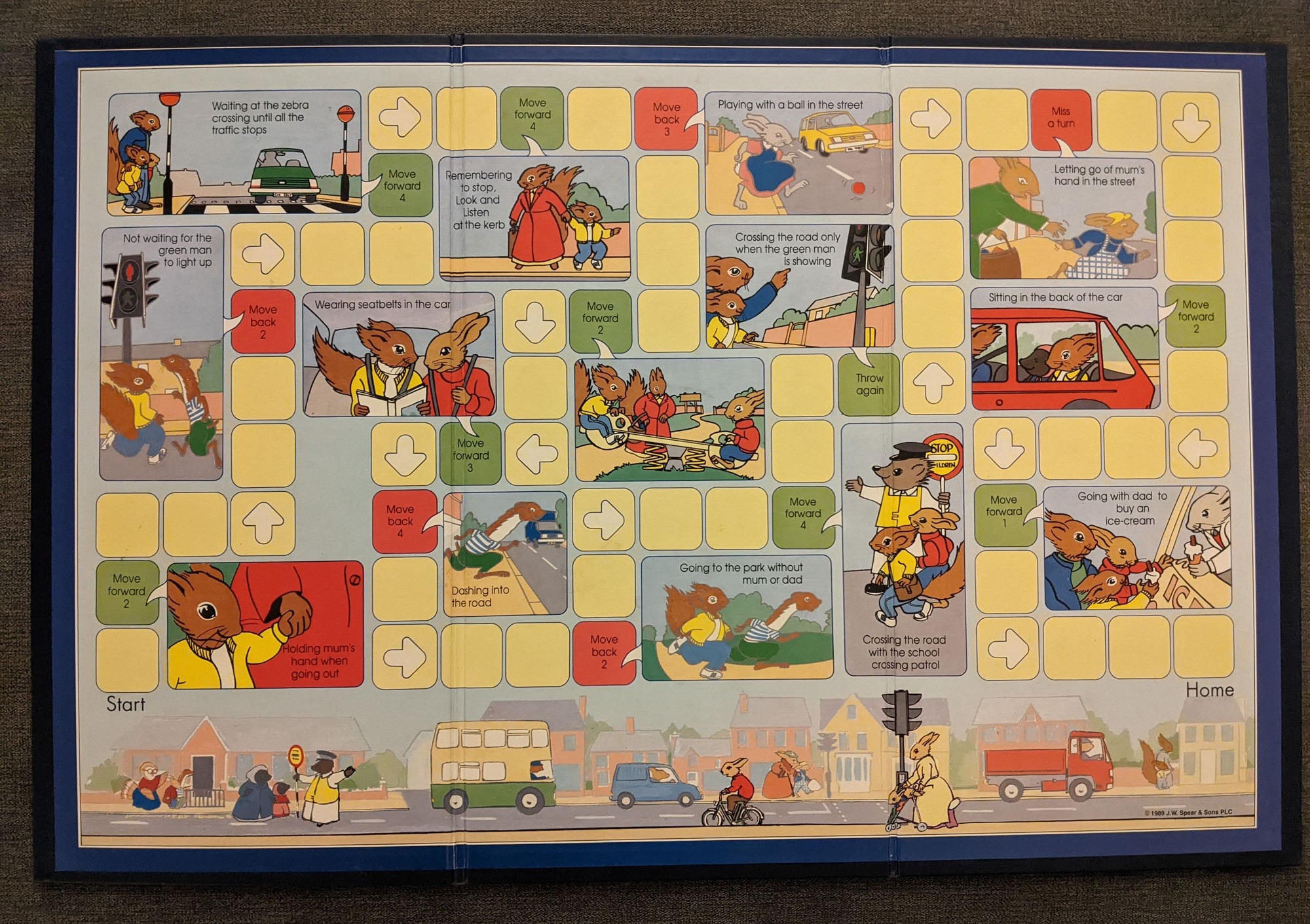
It had been a VERY long time since I’d played Snakes and Ladders or anything similar, and I immediately noticed something that little me never really thought about: there is absolutely no skill involved. The player doesn’t make a single decision throughout the entire game.
This led me to wonder: starting earlier must be the only advantage a player can have, since if two players roll the exact same sequence of numbers, whoever plays first will win, and no player can influence the course of the game. The rules state that the youngest player starts first, so just how much of an advantage does my sister actually have?
To answer this question, we’ll need to think about the game in a slightly different way.
Markov Chains
In the game, the player rolls a die and moves that many spaces forward. Some squares give them a boost forward, and some send them backwards (there are also a couple of other interesting squares, but we’ll talk about that in a moment). The probability each turn of reaching a particular new square is only dependent on where you are at the moment, and once you reach the finish square, you can’t leave it.
Having been going over my Data Science notes during the holiday too, this leapt out to me as a great example of a Markov chain: a random process whose next state depends only on its current state. In fact, it’s more specifically an absorbing Markov chain, one in which every state can reach an absorbing state (a state that cannot be left), in our case the finish square.
Modelling the Game
To model the game as an absorbing Markov chain, we need to define the transition matrix . We’ll consider each square to be a state, with the finish square being the only absorbing state. To calculate the probabilities, we’ll simply work out where each value of the die can take us.
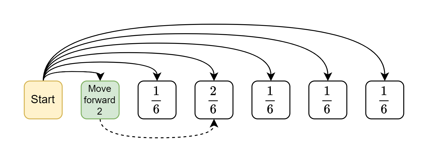
The diagram above shows the probabilities for the first move. There are two ways to get to the middle state, either by rolling a 3 and getting there directly, or by rolling a 1 and getting the boost. These probabilities correspond to the first row of the transition matrix (with all other destination states having a probability of zero).
There are two interesting squares that we need to think about slightly more carefully.
“Throw Again”
One of the squares says “throw again”, so if the player lands on that square, they get another turn immediately. Fortunately, all six squares immediately after this square have no special behaviour - two special squares in one turn would be far too complicated for the game’s target audience of 4-year-olds to handle - so this isn’t too difficult to model.
For each square that can reach the “throw again” square, instead of assigning a probability of to the latter, we instead add to the probability of reaching each of the six squares after it.
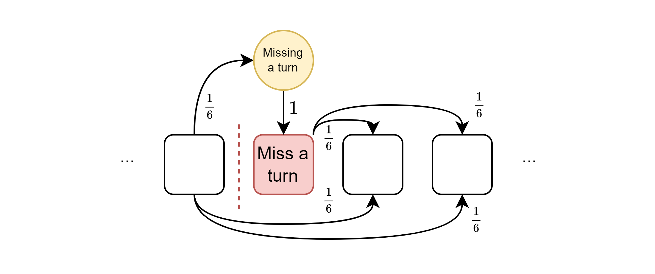
“Miss a Turn”
Another of the squares causes the player to miss a turn. To model this, I decided to add a new “missing a turn” state which is entered instead of the miss a turn square, and which can only transition to the miss a turn square with probability 1.
And with that, we have our transition matrix . We’ll also define to be the submatrix of that excludes the row and column of the absorbing state - yes, the probabilities won’t sum to one, but we’ll see why this is useful in a moment.
The Fundamental Matrix
Now that we’ve defined our absorbing Markov chain, we can find out some very interesting statistics about the game. Let’s begin by working out which squares are more and less likely to be visited.
Intuition
Let’s consider a very simple example.
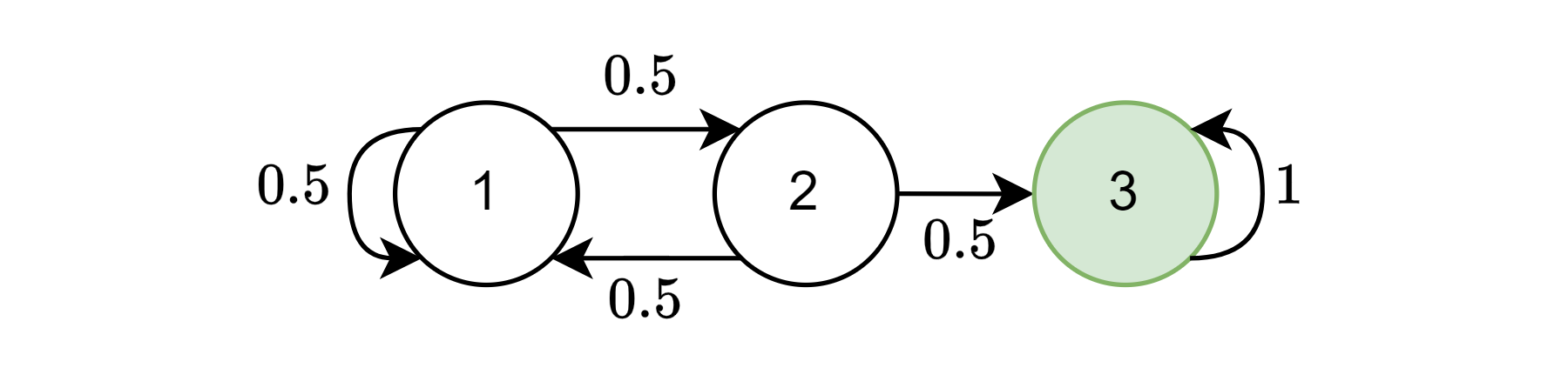
We’ll start by defining and for this example.
We already know that the entries of give the probability of moving from one state to another in one step. But what if we want to know the probability of moving from one state to another in, say, exactly 2 steps? We can do this by summing over all the possible intermediate states:
You’ve probably seen this result before, but we’ve shown that the entries of give the probability of moving from one state to another in exactly 2 steps. We can generalise this to find the probability of moving from one state to another in exactly steps, which is given by .
Let’s look at what happens as gets larger.
After 4 steps, if we started on the left, we have exactly a 50% chance of having been absorbed, and even more than that if we started in the middle. This makes intuitive sense - the middle state is “closer” to the absorbing state (in the sense that it can transition there in one step as opposed to two). After 8 steps, these probabilities have increased even more, and we can see the submatrix tending towards the zero matrix (the proof is left as an exercise to the reader, but it just falls out of the definition of an absorbing Markov chain).
Okay, so why do we need ? Well, we’re about to work out the expected number of times we visit each state (to get an idea of how likely we are to land on each square), but we’ll visit the absorbing state an infinite number of times, so we have to exclude it. Instead, we’ll work out the expected number of times we visit each state before reaching the absorbing state. We know that, since we got rid of the absorbing state from the matrix, no matter and , is the probability of reaching state from state in exactly steps without being absorbed.
Putting it all together
Now it’s time for some real maths. How do we go about finding the expected number of times we visit each state before being absorbed?
First let’s formalise the idea of how many times we visit a state. We’ll define to be the number of times we visit state in some process, where is not the absorbing state. We can write this as
where is an indicator function which is 1 if we are in state at time and 0 otherwise.
Starting in state , we’ll work out the expected number of times we visit state , where neither state is the absorbing state.
As we’ve already established that neither nor are the absorbing state, this final step can use instead of .
Awesome, so represents the expected number of times we visit state starting from state . But that’s a bit awkward to calculate, it’ll only take infinite time to compute!
We could just cut off the computation once the probabilities get small enough, but there’s a trick. This is a geometric series (well, technically a Neumann series, a generalisation), and thanks to the use of instead of , it converges and we can use a formula analogous to that of the sum of a geometric series to get
where is the identity matrix. And there we have it, the long-awaited and hard-earned ✨ fundamental matrix ✨. Let’s call it .
We’ve skipped some fiddly bits (like proving the series even converges - kind of important!), but you can find everything and more in Kemeny and Snell, “Finite Markov Chains” (1960), Chapter 3.
Using the Fundamental Matrix
Let’s not forget why we wanted this in the first place: to find out which squares are more and less likely to be visited. We can do this by looking at the first row of , which gives the expected number of times we visit each state starting from the start square.
Plotting time! Let’s plot the expected number of times we visit each square as a heatmap on the board. The special squares are never visited, as in our model we immediately transition to their corresponding destinations. Really, we’re thinking about the expected number of times we start our turn on each square.
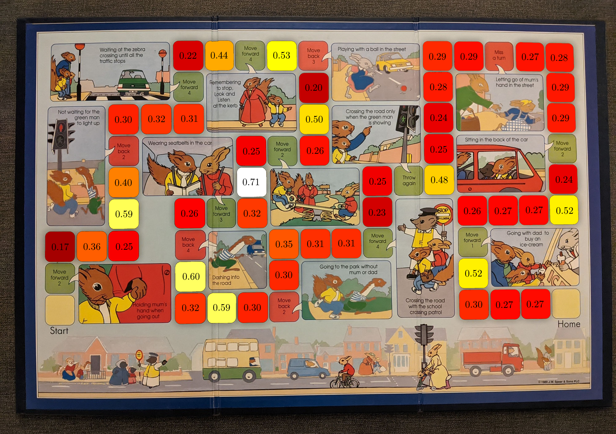
The “hotter” squares are the targets for special squares. The most likely square to be visited is indicated in white, and, looking at the board, it’s not a surprise that it’s the most visited: it’s the target for both square 20’s “move forward 2” and square 26’s “move back 4”!
We can also use the fundamental matrix to find the expected number of turns in the game, or formally, the expected number of steps before being absorbed. This is given by the sum of the first row of :
So, on average, the game lasts about 17 turns. Fun.
Youngest Player Starts
Okay, let’s stop messing around with maths and get to the real question: how much of an advantage does my sister have by starting first?
So far we’ve only considered one lonely and very sad player playing the game by themselves. But what if we have more than one player? Well, as we established right at the start, they can’t interact with each other at all, which gives us the extremely useful property that the number of turns each player takes to finish the game is independent from the others.
Let’s use to denote the number of turns each of the players takes to finish the game. They are independent and identically distributed, drawn from some distribution which we’ll worry about in a moment.
We can then define the event “player 1 wins in turns”, given some number of players , to be
in other words, every player finishes in at least as many turns as player 1.
Then, working out the probability of player 1 winning in any number of turns, given that the s are i.i.d., is easy:
We’ll define player ’s “advantage” over player , , to be the number of times more likely they are to win than player . We’ll also define their “advantage over equality” to be the number of times more likely they are to win than if all players had an equal chance of winning.
But how do we compute all the probabilities in our formula?
The Distribution
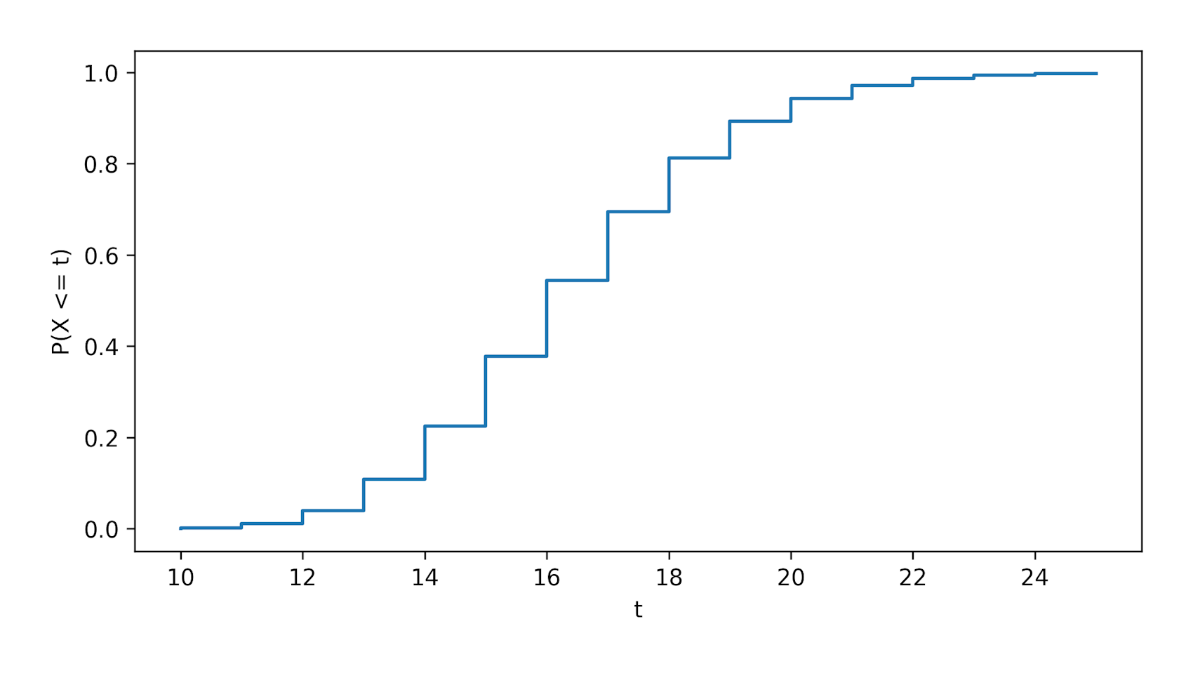
The moment to worry about has come. What is it? Fortunately it’s not too hard to work out. We can calculate the CDF of - the probability of finishing in up to turns - using the transition matrix .
In other words, it’s the probability of transitioning from the start square to the finish square in any number of steps up to , as once we reach the finish square, we can’t leave it.
We also need the PMF - the probability of finishing in exactly turns, which is simply given by the difference in the CDFs:
The Answer
Let’s answer the question. For real this time, we’ve finally done enough maths.
I was playing with my sister and my dad, so . Applying the formulae above - and summing until the probabilities get small enough - we get
That’s nearly 20% more likely than if all players had an equal chance of winning! So, if you’re playing the Road Safety Game, the optimal strategy is to be the youngest player. Very useful indeed.
What about the other players’ chances?
Time for a bit more maths. We can’t end the post without a nice colourful plot.
How can we calculate , the probability that an arbitrary player wins? In order for them to win on a specific turn, all the players who play before them must not yet have finished (i.e. finish in strictly more turns than them), but the players who play after them may finish that turn or later.
That’s a lot of symbols, so let’s plot it for , the numbers of players the box says the game is for.
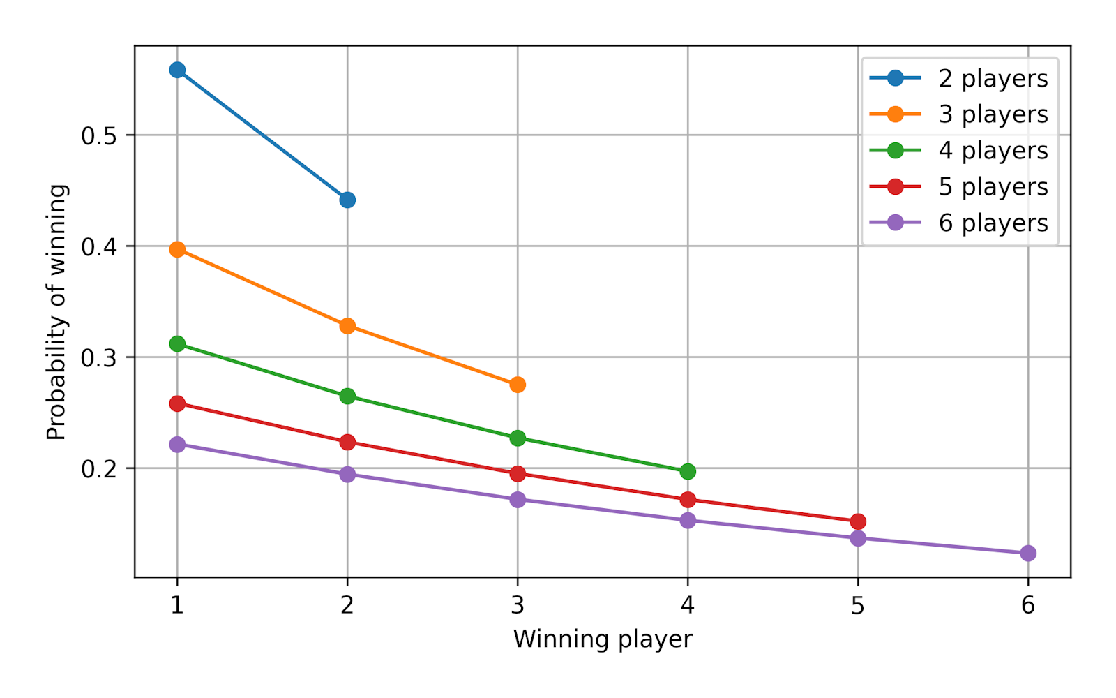
As we might expect, the earlier you play in the sequence, the more likely you are to win. Let’s look at the advantage of the youngest player over equality, the second player, and the last player, for .
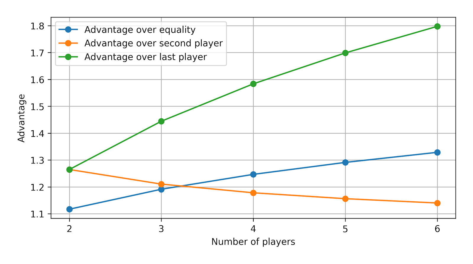
It’s interesting that, while the youngest player’s advantage over equality and over the last player increases with , their advantage over the second player decreases.
Conclusion
Wow, that’s been a lot of maths. I am very much counting this as 10 hours of Data Science revision - in my defence, I’m pretty sure half of what I’ve done here is examinable. I initially used an empirical approach to work out the probabilities, but I’m glad I went back and did it properly because it’s much more satisfying to have a nice formula.
My New Year’s resolution is to do more interesting stuff outside of compulsory work, so hopefully this is the first of many interesting posts to come!
I hope you’ve enjoyed reading this post and maybe learnt something new? Please feel free to share it with anyone you think might be interested, and let me know if you have any questions or comments!